Design of data acquisition and processing system involves deciding whether the data collected will be analyzed by analog or digital techniques.
- Analog
- Digital
- Hybrid system
Analog System Devices which produce or directly process signals that vary in a continuous manner and can assume an infinity of values in any given range.
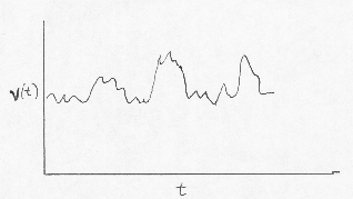
some examples of analog devices: mercury-in-glass thermometers, strain gages and hot wires.
Digital System Devices which produce or directly process signals or data which vary in discrete steps.
e.g.
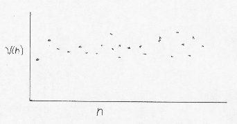
Some examples of digital devices: Switches and most types of Mechanical or electronic counters
In many applications the instrumentation for a particular measurement system can be best implemented using devices which are analog, digital or both i.e. Hybrid Systems.
Advantages of Digital Instrumentation
- higher accuracy and analysis speed
- difficult to design and build analog electronics which are immune to external influences (e.g. electrical and electro-magnetic noise, temperature variation, etc.)
- Availability of algorithms for fast computations of discrete Fourier transformations on the digital computer (FFT)
- Availability of low-cost general purpose digital computers and various interfaces
- Low cost (compare hard wire FFT vs. PC with A/D board)
- Programmed to perform more functions
- Give results with higher accuracy
- Order of magnitude slower than hard-wired systems but speed is generally adequate
- More versatile than hard-wired logic systems since logic functions can be easily altered by just changing software
- Systems are now available which combine advantages of each.
Roughly Organized into three categories
- Measurement process model is not known, and many times the quantities being measured may not be well understood. Thus, measurement is the gathering of sufficient data in an attempt to construct a model of the unknown.
- Testing and Calibration device is being checked against its design standards or measurements of certain parameters. Variables to be measured and requirements for accuracy and precision have been established earlier and are known prior to test and/or calibration.
- Control System initiates a series of actions measures them and then takes corrective action if the desired results are not achieved.
Most important question What sort of information is ultimately going to be extracted from the data acquired? What processing functions are going to be applied to the data?
We will talk about this later if time permits.
a) Overall Features and Capabilities
The following series of questions should be addressed.
- # of channels for proposed work.
- Can number of channels be easily increased and if so how will such an expansion affect other power system performance specifications such as acquisition speed, power supply capability, portability, etc?
- What types of transducers will be used and what are there output ranges, output impedances, signal conditioning requirements, etc.?
- What peripherals or options will be required to implement a complete operational data acquisition system with the desired capabilities?
- What performance boosting options might be desirable. e.g. floating point processor
b) Accuracy - must decide beforehand what desired accuracy is so that educated choices can be made with regard to what transducers, signal conditioners, A/D and D/A converters should be used.
- must assess speed vs. accuracy requirements as well a factoring in cost.
c) Acquisition Speed
- Low-speed: < 1 sample/sec
- intermediate speed: 100 samples/sec 1000 samples/sec
- High speed: > 1000 samples/sec
d) Data Storage Compatibility should insure that medium used for storage (mag tapes or disks) of the data (and transferring) be compatible, both with respect to the physical medium and to the format of the data created by the user or the operating system software.
With the increasing use of local computer net working this problem has been partially alleviated because collected data can be transferred between computer systems through the network without using a physical transfer medium.
e) System Portability when data acquisition and control systems are required in the field, electric generators can be used as well as lightweight, battery-powered systems.
f) Total System and Operating Cost range $500 up to several hundred thousand dollars.
General Considerations for A/D Conversion
A/D provides a series of numbers each of which corresponds to the weighted intergral of the analog signal over some time period, DS, called the aperture which is less than or equal to the sampling period D
\ if u(t) is the signal and un
is the digital sample

where m is the quantization noise.
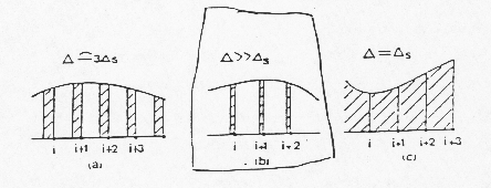
A/D Converter output corresponds to the shaded area in the figure.
Generally DS/D
<< 1 so that a convenient continuous approximation to the sampled
signal is:
![]()
where d represents the impulse function.
From this the time average of u0(t) is the average of the numbers
generated by the A/D, i.e.

but N = T/D = # of samples
\
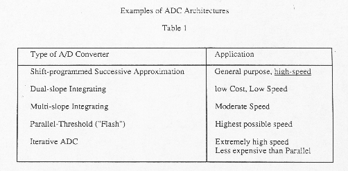
Representative Types of Analog-to-Digital Converters
Only inherent advantage of successive Approximation ADCs is speed. In all other respects the integrating ADC is superior i.e., cost and reliability.
Quantization Errors
Arise from the approximation of a continuos signal by a finite set of numbers. In an ideal ADC, m is the difference between the value of the analog signal and the digital output due to the finite resolution of A/D.

The quantization error m acts as a noise and is introduced by the sampling process. How does one minimize affect? Must insure that enough Gain is applied to the input signal so that the voltage levels are sufficiently above the quantization noise.
Alternately, a higher Resolution A/D converter can be used to reduce the quantization noise to Acceptable levels (i.e. more bits in A/D).
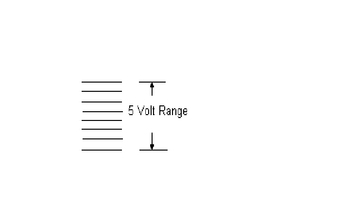
3 bit A/D e.g. 23 levels can resolve to 5/8th ± ½ LSB
What if a signal is less than 5/8 volt? Must provide gain to use
more of the range of ADC and/or use ADC with more bits.
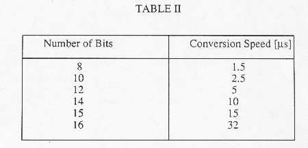
ADC Resolution versus Typical Conversion Speed
Clipping Errors
Clipping errors can arise from the fact that the A/D converter has a finite range.
Examine the previous figure; the range is [O,R] and the sampled signal is shown to be clipped at those values.
Many of the commercially available A/Ds have selectable settings for
R.
e.g.
| unipolar ® | 0 ± 5 Volts |
| 0 ± 10 Volts | |
| bipolar ® | -5 ± 5 Volts |
| -10 ± 10 Volts |
Most insure that all voltages in the input signal are within the range
of the A/D (i.e., may need to precondition signal)
The Sampling Rate
Requirements for high speed, high accuracy and low cost are mutually
exclusive \ the sampling rate/accuracy trade-off
can be very important in the selection of an A/D converter. Like the choices
outlined above for quantization and clipping problems the correct or optimal
sampling rate is very much a function of the particular experiment and
of the type of processing that will be carried out on the sample data.
e.g.

UN is the estimate of the mean
U is the true mean
var<U> is the true variance of the fluctuating signal
N samples must be statistically independent.
\ if only probability analysis is required there can be considerable savings in data storage requirements and A/D hardware complexity is reduced because the A/D speeds are much lower.
i.e. No sense in sampling fast because samples wont be statistically independent.
Sampling for a time series analysis involves an entirely different set of sampling constraints if spectral analysis or time reconstruction of the signals is to be carried out.
Basic Problem: Folding or Aliasing
The phenomenon of aliasing does not occur if the rate at which the signal is sampled is at least twice the highest frequency. In fact, all of the information present in the original signal is also present in the digitized signal. this is not the case if the signal is aliased.
This fact is the essence of the Shannon Sampling Theorem.
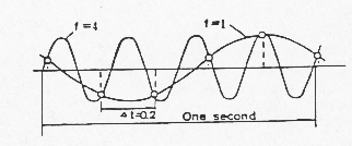
Aliasing of 4Hz sine wave to a 1Hz sine wave by a 5Hz sampling rate.
It is not always convenient to sample at rates higher than twice the highest frequency because of the need to have long time records to insure that the lowest frequencies are captured \ must precondition signal by analog low-pass filtering prior to sampling.
An illustration of aliasing
1) ![]() where
where 
p integer
q fractional part < 1
T Sampling interval
let T = .005 sec and f0 = 1025 Hz

![]()
![]()
substitute ![]() and
and  in
equation 1.
![]() =
= 
= ![]()
= ![]()
= ![]()
because ![]() for all i.
for all i.
There are now two possibilities depending on whether p is even or odd:
1. p even, ![]() for all I
for all I
![]()
2. p odd, ![]()
in the first case for p even

Þ effective frequency is 
In the above example p is 10 which is even hence the reduced frequency is (0.25)(100) = 25 Hz. \ A sine wave of frequency = 1025 Hz when sampled at interval T = .005 sec or 200 samples/sec would be indistinguishable from a sine wave at 25 Hz.
The frequency (1/2T) plays a special role in digital data so hereafter it is designated by F (for folding).
Now F = (1/2T) = (S/2) where S is the sampling rate. (This is called the Nyquist folding frequency.)
Back to the second case, p odd
![]()
![]()
![]()
in this case:

![]()
\ odd cases are referenced to the folding
frequency where as even to 0 Hz.
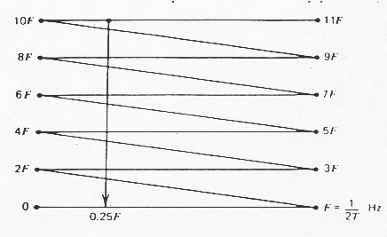
The first 11 pleats of a Nyquist aliasing diagram.
From example: 1025 Hz with sampling rate 200 samples/sec 10.25 F appears as 0.25 F would 1.75 F, 2.25 F, 3.75 F, 4.25 F, 5.75F, 6.25 F, 7.75 F, 8.25 F, 9.75 F, etc.