Why study probability and statistics
- Random phenomena, e.g., Turbulence, Random Acoustic Waves, Random Vibrations, Statistical Thermodynamics and etc.
- Measurement Uncertainty
- Statistical Process Control (SPC) and Design Experiments
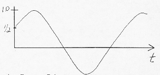
- Deterministic Process Behavior at one or several times determines behavior for all times.
- Example of deterministic process: Suppose we have a wave and further suppose that at t = 0, f (0) = ½, f(0) > 0
- Random Process Behavior at any time can be (not necessarily) statistically independent of behavior at any other time. We could say that behavior is only correlated for short times (or spatial distance) and becomes increasingly uncorrelated as the time (or spatial distance) in increased.
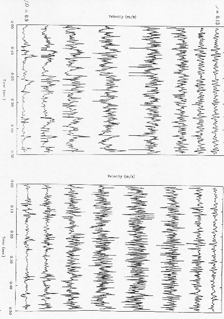
- Example of a Random process, Velocity Field in a turbulent jet. Note that the flow is random and these results are not due to random scatter in the data values.


- What Statistical Quantities have physical relevance? Mean Values, Standard Deviations, Probability Density Functions or Histograms (e.g. Gaussian), Spectra and Correlation Functions.
- Mean Values, Time average or Ensemble average
Time Average of Mean Value

Ensemble Average of Mean Value

- Standard Deviations, Time average or Ensemble average

Ensemble Average

- Central Tendency Tendency towards one central value about which all other values are scattered. I.e., concept of mean value standard deviation and higher moments.
- Probability Particular interval of values for a random variable are measured at some frequency relative to any other random variable. Leads to the concept of a histogram and frequency distribution. Ultimately leads to probability density function, p(x)
Two examples which demonstrate how to compute a histogram and frequency distribution follow.
Example from Text: 4.1 pg. 128
Table from text: 4.1 pg. 127: Sample of variable x
Figure from text: 4.2 pg. 128: Histogram and frequency distribution for data in Table 4.1

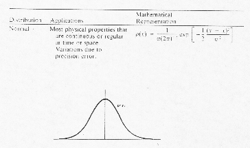
- Infinite Statistics, assume for now Gaussian or Normal Distribution:
The probability, P (x), that random variable, x, will
assume a value within the interval ![]() ,
is given by the area under p (x). This is written as
,
is given by the area under p (x). This is written as

We can simplify the integration by transforming to a different set of
variables. If we write ![]() ,
as the standardized normal variable for any x, and
,
as the standardized normal variable for any x, and ![]() ,
as the z variable which specifies an interval on
,
as the z variable which specifies an interval on ![]() so
that the above equation becomes:
so
that the above equation becomes:

The value in the square brackets is known as the normal error function and provides ½ the probability over the entire interval. This half value is tabulated in the following table.
Table from text: 4.3 pg. 135: Probability Values for Normal Error
Example from text: 4.2 pg. 135
Figure from text: 4.3 pg. 134: Integration terminology for the normal error function.
Figure from text: 4.4 pg. 136: Relationship between the probability density function and its statistical parameters x and s for a normal distribution.
Example from text: 4.3 pg. 137
Finite Statistics
In real life we deal with finite samples, hence we need to try and quantify how well we know the mean from the finite sample N. Keep in mind that finite statistics describe only the behavior of the finite data set.
- We define a sample mean as

and the sample variance as

where
- The predictive utility of infinite statistics can be extended to data sets of finite samples size with a few changes. The sample variance can be weighted in such a manner so as to correct for the finite sample of the measured. Lets assume a Normal Distribution and write:
- Standard Deviation of the Means Imagine a though experiment where you measure a particular variable N times under fixed operating conditions. Now repeat this same experiment M times. For each experiment we will obtain value which will in general be different than any other estimate because of the finite sample.
The amount of variation in our individual estimate of the mean should
depend on the sample variance ![]() and
the number of samples N. The standard deviation of the mean,
and
the number of samples N. The standard deviation of the mean, ![]() can be shown to behave as:
can be shown to behave as:

Figure from text: 4.6 pg. 141: Relationships
between Sx and a distribution of x and between ![]() and
the true value of x.
and
the true value of x.
The standard deviation of the means represents a measure of the precision in a sample mean. The rang over which the possible values of the true mean value might lie at some probability level, P can be written as:
![]()
so ![]() represents a precision interval at the assigned probability (P%)
within which one should expect the true value of x to fall. Thus
we write the estimate of the true mean value based on a finite data set
as
represents a precision interval at the assigned probability (P%)
within which one should expect the true value of x to fall. Thus
we write the estimate of the true mean value based on a finite data set
as
![]()
Example from Text: 4.4 pg. 141
Numbers of Measures Required
How many measurements, N, are required to give an acceptable precision
in the mean value? The precision interval, CI is estimated by:

Where Sx is a conservative estimate based on prior
experience. Remember that the precision interval is two-sided about ![]() \
define
\
define  and
and  .
.
The accuracy of this equation depends on how well Sx2
approximates s2. The problem
is that an estimate for the sample variance is needed. A way around this
is to make a few measurements N, to obtain an estimate of the sample
variance that we call S1. The use S1
to estimate the number of estimates required.

This establishes that ![]() additional measurements will be needed.
additional measurements will be needed.
Example from Text: 4.12 pg. 161
Example from Text: 4.13 pg. 151